The purpose of this post is to understand how linear regression works in order to start learning Machine Learning. Linear regression is the easiest one to understand Machine Learning. I used python for the implementation. I’m new to python and the source code may not look good for python programmers but I hope you can understand what I want to do in the code. I prepared Dockerfile so you can easily try it yourself without building environment.
The versions that I used are following.
| Module | version |
|---|---|
| python | 3.9.1 |
| numpy | 1.20.1 |
| matplotlib | 3.3.4 |
| seaborn | 0.11.1 |
Understanding how to get the linear line by calculation
The data which we take this time is 2 dimensional data. There’s relationship between X and Y. Therefore, the formula which we want to get is following.
$$ y = x * w + b $$
w is weight and b is bias. The image looks like this.
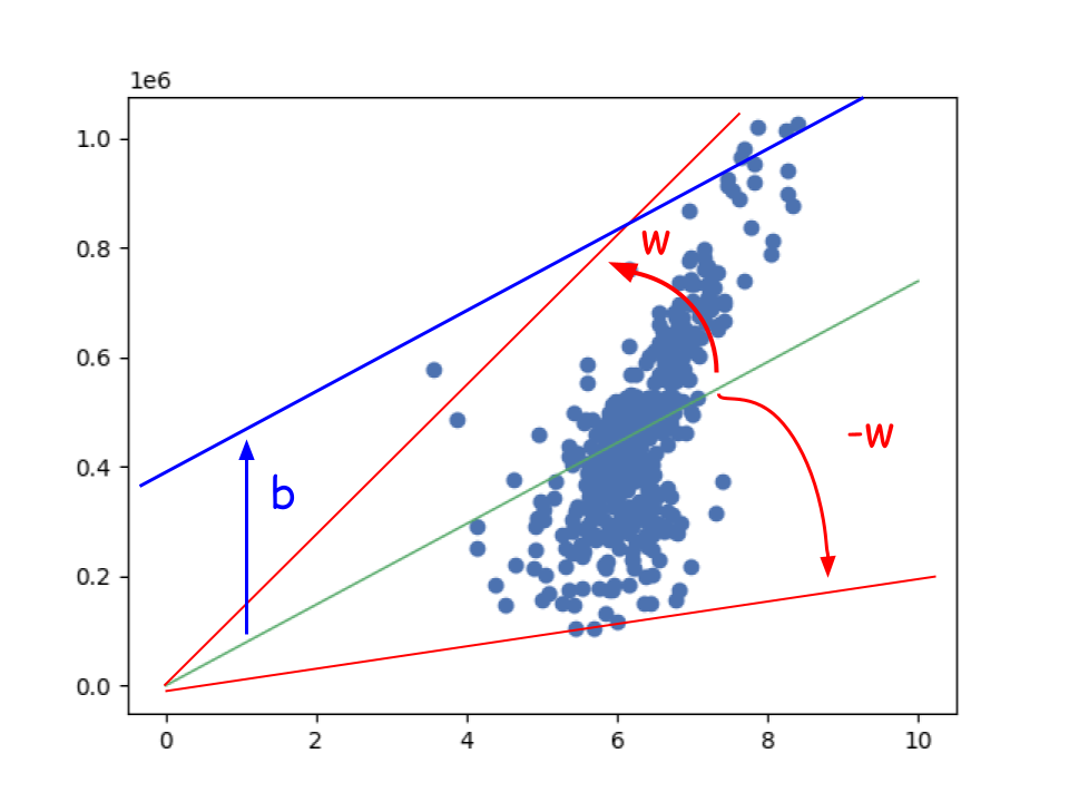
The bigger value the w is, the steeper tha line becomes but we can’t get the proper line with only w because data doesn’t necessarily start from 0. So we need to get bias too. Machine Learning is all about to derive the weight and bias. When there are multiple elements the dimensions is also more than 3 dimensions.
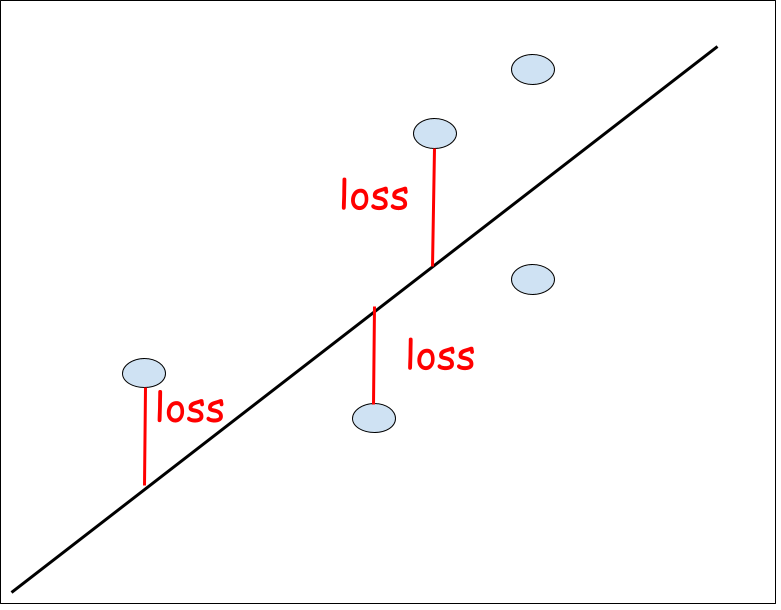
To get the line which fits the data, we need to calculate sum of loss for all elements. The sum of the loss of the most fitting line is the smallest. To get the loss, we need a start line. From here, we will get the loss by changing weight and bias. If the total loss is smaller than previous line, we will take the weight and bias for the candidate. By repeating the process, its value converge. The speed to converge depends on the learning rate. If the learning rate is small enough the result will be more precise. If it is big the loss value may not converge because it jumps over the minimum point.
We can calculate the loss with following formula.
$$ L = \frac{1}{m} ((wx + b) – y) ^ 2 $$
We can simply get the sum but it becomes very big if there are bunch of data. Therefore, we use average here. Value needs to be squared since the loss can be minus value. Let’s try to implement this with python code.
Simple implementation without bias
Let’s set 0 to bias first to make the code easier. The function to calculate loss looks like this. np is numpy module. Both X and Y are array.
def calculateLoss(X, Y, weight, bias = 0):
    predictedLine = X * weight + bias
    return np.average((predictedLine - Y) ** 2)
This is train function which repeats the training process. As I mentioned above, we need to change weight value and evaluate the result. This function repeats the process 1000 times and the learning rate is set to 100.
def train(X, Y):
weight = 0
learningRate = 100
for i in range(1000):
if i % 50 == 0:
plot.plot(X, Y, "bo")
image = plot.plot(
[0, 10],
[0, 10 * weight],
linewidth = 1.0,
color = "g")
images.append(image)
currentLoss = calculateLoss(X, Y, weight)
print(i, currentLoss)
if currentLoss > calculateLoss(X, Y, weight + learningRate):
weight += learningRate
elif currentLoss > calculateLoss(X, Y, weight - learningRate):
weight -= learningRate
else:
return weight
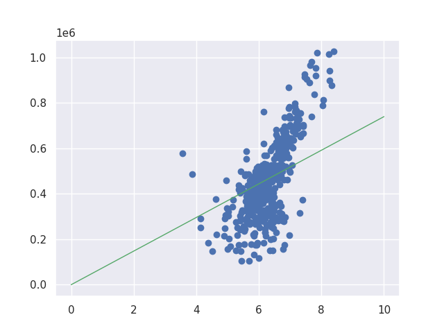
return weightI don’t show the code to save the images but you can check it in my GitHub repository if you want. The result looks like this. As you can see from the gif image at right side, the code improves the line to fit the data. The end result looks good if we draw a line from 0.
Introducing bias to the calculation
We understood how it works without bias parameter. Next step is to introduce bias parameter to fit the line to the data points. I implemented two functions in order to compare them. In the first implementation it immediately evaluates the result when it calculates the loss with one parameter change. This is the code.
def trainWithBias1(X, Y):
    weight = 0
    bias = 0
    learningRate = 50
    for i in range(20000):
        currentLoss = calculateLoss(X, Y, weight, bias)

        if i % 200 == 0:
            plot.plot(X, Y, "bo")
            image = plot.plot(
                [0, 10],
                [0 + bias, 10 * weight + bias],
                linewidth = 1.0,
                color = "g")
            images1.append(image)
            print(i, weight, bias, currentLoss)

        if currentLoss > calculateLoss(X, Y, weight + learningRate, bias):
            weight += learningRate
        elif currentLoss > calculateLoss(X, Y, weight - learningRate, bias):
            weight -= learningRate
        elif currentLoss > calculateLoss(X, Y, weight, bias + learningRate):
            bias += learningRate
        elif currentLoss > calculateLoss(X, Y, weight, bias - learningRate):
            bias -= learningRate
        else:
            return (weight, bias)

    return (weight, bias)
On the other hand, second one prepares all results first and then it picks the best one by comparing the results. It looks like this below.
def trainWithBias2(X, Y):
    weight = 0
    bias = 0
    learningRate = 50
    for i in range(20000):
        currentLoss = calculateLoss(X, Y, weight, bias)
        loss1 = calculateLoss(X, Y, weight + learningRate, bias)
        loss2 = calculateLoss(X, Y, weight - learningRate, bias)
        loss3 = calculateLoss(X, Y, weight, bias + learningRate)
        loss4 = calculateLoss(X, Y, weight, bias - learningRate)

        if i % 200 == 0:
            plot.plot(X, Y, "bo")
            image = plot.plot(
                [0, 10],
                [0 + bias, 10 * weight + bias],
                linewidth = 1.0,
                color = "g")
            images2.append(image)
            print(i, weight, bias, currentLoss)

        minLoss = min(currentLoss, loss1, loss2, loss3, loss4)
        if minLoss == loss1:
            weight += learningRate
        elif minLoss == loss2:
            weight -= learningRate
        elif minLoss == loss3:
            bias += learningRate
        elif minLoss == loss4:
            bias -= learningRate
        else:
            return (weight, bias)

    return (weight, bias)
Most people may not be interested in the result though its process is a bit different… The column is respectively iteration, weight, bias, loss. Second implementation is a bit better than first one but its performance is worse than first one.
| trainWithBias1 | trainWithBias2 |
| … 1600 74750 -5250 18568893742.920372 1800 76100 -13900 18450116406.20223 2000 77500 -22500 18333523775.166157 2200 78850 -31150 18217856466.314728 2400 80250 -39750 18104422970.0625 2600 81600 -48400 17991865689.07779 2800 82950 -57050 17880917189.31354 3000 84350 -65650 17772144074.491417 … 16400 176050 -643950 14023883638.344421 | … 1600 74650 -5350 18568104283.896935 1800 76000 -14000 18449542016.327198 2000 77350 -22650 18332588529.97792 2200 78750 -31250 18217183862.605446 2400 80100 -39900 18103340404.122883 2600 81500 -48500 17991094871.534252 2800 82850 -57150 17880361440.91841 3000 84200 -65800 17771236791.523026 … 16400 176050 -643950 14023883638.344421 |
I show only one result because both end results are the same. The line seems to be fitting to the data. If we change the learning rate to smaller value its result may change a bit but I stop here because I understood how it works. If you are interested in it you can try it yourself.

Improving the implementation by gradient decent
The previous way is good way to understand how it works but its accuracy depends on the learning rate. If the learning rate is big the value converges faster but it is less precise. If the learning rate is smaller value its result is more precise but it takes longer time. A better way is to jump a lot as long as the goal is far away and walk slowly when the goal is almost there.
We calculated the sum of the loss by squaring the difference. Its diagram looks like this.
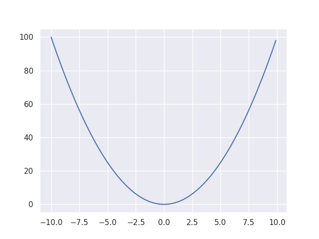
X axis is weight and Y axis is loss. When the loss is big its gradient is large. When the loss is 0 its gradient is also 0. It means if we introduce gradient value to learning rate we can achieve what we want to do that I explained above. This way is called gradient decent. Let’s see the formula again.
$$ L = \frac{1}{m} ((wx + b) – y) ^ 2 $$
Let’s differentiate it respectively with respect to $w$ and $b$ without $\frac{1}{m}$.
$$ \begin{eqnarray}
((wx + b) – y) ^ 2 &=& (wx + b)^2 – 2y(wx + b) + y^2 \\
&=& (wx)^2 + 2wxb + b^2 – 2xyw – 2yb + y^2 \\
\frac{ \partial L }{ \partial w } &=& 2wx^2 + 2xb – 2xy \\
&=& 2x(wx + b – y) \\
\frac{ \partial L }{ \partial b } &=& 2wx + 2b – 2y \\
&=& 2(wx + b – y)
\end{eqnarray}$$
Let’s put $\frac{1}{m}$ back in it again. Because we need total loss I putted $\sum_{i=1}^{n}$.
$$ \begin{eqnarray}
\frac{\partial L}{\partial w} &=& \frac{2}{m} \sum_{i=1}^{m} x_i(wx_i + b – y_i) \\
\frac{\partial L}{\partial b} &=& \frac{2}{m} \sum_{i=1}^{m} (wx_i + b – y_i)
\end{eqnarray}$$
OK, it looks easy to implement it. The following function is to get gradients for weight and bias.
def getGradient(X, Y, weight, bias = 0):
    weight_loss = X * (X * weight + bias - Y)
    bias_loss = (X * weight + bias - Y)
    weight_gradient = 2 * np.average(weight_loss)
    bias_gradient = 2 * np.average(bias_loss)
    return (weight_gradient, bias_gradient)
Train function looks like this.
def trainByGradientDecent(X, Y):
weight = 0
bias = 0
learningRate = 0.01
for i in range(20000):
(weight_gradient, bias_gradient) = getGradient(X, Y, weight, bias)
weight -= weight_gradient * learningRate
bias -= bias_gradient * learningRate
if i % 200 == 0:
plot.plot(X, Y, "bo")
image = plot.plot(
[0, 10],
[0 + bias, 10 * weight + bias],
linewidth = 1.0,
color = "g")
images.append(image)
print(i, weight, bias)
if weight_gradient == 0 and bias_gradient == 0:
return (weight, bias)
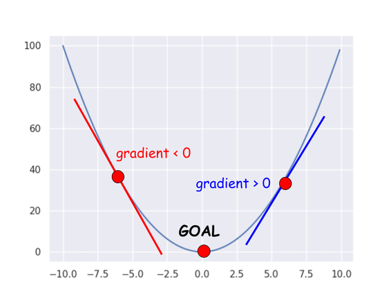
return (weight, bias)Look at the line 7 and 8. The value is subtracted because the direction of the gradient at current position is opposite value against the goal. If current position is left side in the following image it should go to the right side. If it’s right side it should go to the left side. That’s why we need to subtract the result.
When I set 50 to the learning rate the value got overflow and I god following error message.
$ bash start.sh
/usr/local/lib/python3.9/site-packages/numpy/core/_methods.py:178: RuntimeWarning: overflow encountered in reduce
  ret = umr_sum(arr, axis, dtype, out, keepdims, where=where)
/src/gradient_decent.py:19: RuntimeWarning: invalid value encountered in double_scalars
  weight -= weight_gradient * learningRate
So I changed the learning rate several times.
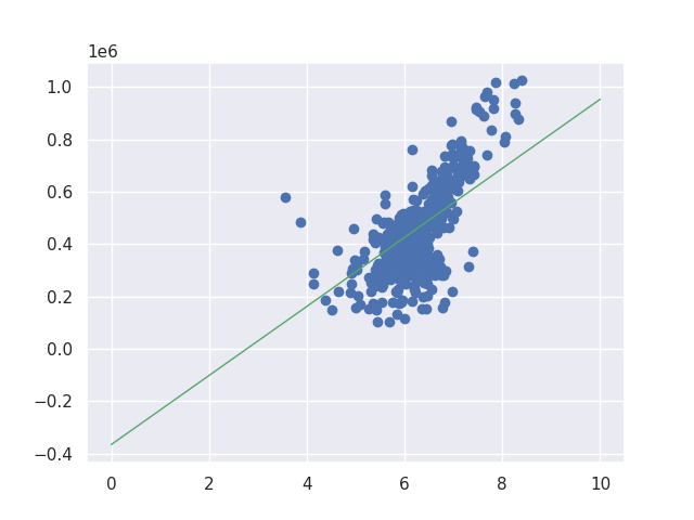
learning rate = 0.001, iteration = 40000 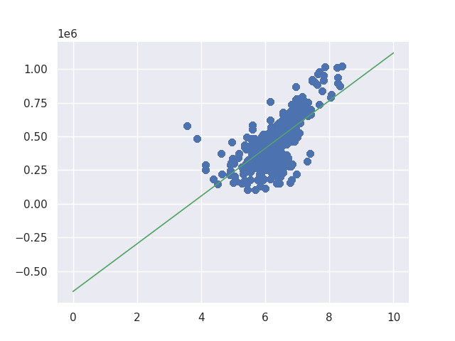
learning rate = 0.01, iteration = 20000
There is still room for improvement when learning rate is 0.001. I needed to increase the iteration for learning rate 0.001 to get the similar result to learning rate 0.01. If we changed the iteration to 100000 we can get following result.
Linear regression by numpy module
The last thing I want to confirm is how accurate the result is. We can derive the line by using numpy module as well. So I looked for how to do that and implemented it. It was very easy to use. Following code is complete code but main process is done by 2 lines (line 10 and 11). I copied the code from official API reference. Other code is the same as others.
import matplotlib.pyplot as plot
import matplotlib.animation as animation
import numpy as np
import seaborn as sns

data = np.genfromtxt('./dataset/housing.csv', delimiter = ',', skip_header = 1)
X = data[:, 0]
Y = data[:, 3]

X2 = np.vstack([X, np.ones(len(X))]).T
weight, bias = np.linalg.lstsq(X2, Y)[0]

sns.set()
plot.xticks(fontsize = 10)
plot.yticks(fontsize = 10)
plot.xlabel("RM", fontsize = 10)
plot.ylabel("MEDV", fontsize = 10)

plot.plot(X, Y, "bo")
plot.plot([0, 10], [0 + bias, 10 * weight + bias], linewidth = 1.0, color = "g")
plot.savefig("/src/images/linear-regression-by-numpy.png")
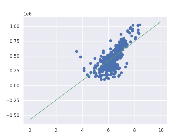
The result looks like this below. Right side is the result by numpy function. They are almost the same. If we increase the iteration it will be more precise.
learning rate = 0.001, iteration = 100000 
numpy
End
We learnt how linear regression works. We understood how to calculate the loss by comparing results but gradient decent is more efficient. So we derived the desired equation and implemented it. Its result is almost the same as the numpy function. This is the very basics for Machine Learning but at least I could enjoy the process that my code was approaching to the desired line. We can step up to the next level.
If you are interested in machine learning following book is super good because it explains how it works in detail. The author explains math for machine learning but it’s clear explanation.


Comments